Building a Kimball dimensional model with dbt
Dimensional modeling is one of many data modeling techniques that are used by data practitioners to organize and present data for analytics. Other data modeling techniques include Data Vault (DV), Third Normal Form (3NF), and One Big Table (OBT) to name a few.
While the relevance of dimensional modeling has been debated by data practitioners, it is still one of the most widely adopted data modeling technique for analytics.
Despite its popularity, resources on how to create dimensional models using dbt remain scarce and lack detail. This tutorial aims to solve this by providing the definitive guide to dimensional modeling with dbt.
By the end of this tutorial, you will:
- Understand dimensional modeling concepts
- Set up a mock dbt project and database
- Identify the business process to model
- Identify the fact and dimension tables
- Create the dimension tables
- Create the fact table
- Document the dimensional model relationships
- Consume the dimensional model
Dimensional modeling
Dimensional modeling is a technique introduced by Ralph Kimball in 1996 with his book, The Data Warehouse Toolkit.
The goal of dimensional modeling is to take raw data and transform it into Fact and Dimension tables that represent the business.
The benefits of dimensional modeling are:
- Simpler data model for analytics: Users of dimensional models do not need to perform complex joins when consuming a dimensional model for analytics. Performing joins between fact and dimension tables are made simple through the use of surrogate keys.
- Don’t repeat yourself: Dimensions can be easily re-used with other fact tables to avoid duplication of effort and code logic. Reusable dimensions are referred to as conformed dimensions.
- Faster data retrieval: Analytical queries executed against a dimensional model are significantly faster than a 3NF model since data transformations like joins and aggregations have been already applied.
- Close alignment with actual business processes: Business processes and metrics are modeled and calculated as part of dimensional modeling. This helps ensure that the modeled data is easily usable.
Now that we understand the broad concepts and benefits of dimensional modeling, let’s get hands-on and create our first dimensional model using dbt.
Part 1: Setup dbt project and database
Step 1: Before you get started
Before you can get started:
- You must have either DuckDB or PostgreSQL installed. Choose one, and download and install the database using one of the following links:
- Download DuckDB
- Download PostgreSQL
- You must have Python 3.8 or above installed
- You must have dbt version 1.3.0 or above installed
- You should have a basic understanding of SQL
- You should have a basic understanding of dbt
Step 2: Clone the repository
Clone the github repository by running this command in your terminal:
git clone https://github.com/Data-Engineer-Camp/dbt-dimensional-modelling.git
cd dbt-dimensional-modelling/adventureworks
Step 3: Install dbt database adaptors
Depending on which database you’ve chosen, install the relevant database adaptor for your database:
# install adaptor for duckdb
python -m pip install dbt-duckdb

# OR

# install adaptor for postgresql
python -m pip install dbt-postgres
Step 4: Setup dbt profile
The dbt profile (see adventureworks/profiles.yml) has already been pre-configured for you. Verify that the configurations are set correctly based on your database credentials:
adventureworks:
  target: duckdb # leave this as duckdb, or change this to your chosen database

  # supported databases: duckdb, postgres
  outputs:
    duckdb:
     type: duckdb
     path: target/adventureworks.duckdb
     threads: 12

    postgres:
      type: postgres
      host: localhost
      user: postgres
      password: postgres
      port: 5432
      dbname: adventureworks # create this empty database beforehand
      schema: dbo
      threads: 12
Step 5: Install dbt dependencies
We use packages like dbt_utils in this project, and we need to install the libraries for this package by running the command:
dbt deps
Step 6: Seed your database
We are using dbt seeds (see adventureworks/seeds/*) to insert AdventureWorks data into your database:
# seed duckdb
dbt seed --target duckdb

# seed postgres
dbt seed --target postgres
Step 7: Examine the database source schema
All data generated by the business is stored on an OLTP database. The Entity Relationship Diagram (ERD) of the database has been provided to you.
Examine the database source schema below, paying close attention to:
- Tables
- Keys
- Relationships
Step 8: Query the tables
Get a better sense of what the records look like by executing select statements using your database's SQL editor.
For example:
select * from sales.salesorderheader limit 10;
Output:
┌──────────────┬──────────────┬─────────────────┬───┬───────────────┬─────────────────────┬────────────────┐
│ salesorderid │ shipmethodid │ billtoaddressid │ … │ salespersonid │      shipdate       │ accountnumber  │
│    int32     │    int32     │      int32      │   │     int32     │      timestamp      │    varchar     │
├──────────────┼──────────────┼─────────────────┼───┼───────────────┼─────────────────────┼────────────────┤
│        43659 │            5 │             985 │ … │           279 │ 2011-06-07 00:00:00 │ 10-4020-000676 │
│        43660 │            5 │             921 │ … │           279 │ 2011-06-07 00:00:00 │ 10-4020-000117 │
│        43661 │            5 │             517 │ … │           282 │ 2011-06-07 00:00:00 │ 10-4020-000442 │
│        43662 │            5 │             482 │ … │           282 │ 2011-06-07 00:00:00 │ 10-4020-000227 │
│        43663 │            5 │            1073 │ … │           276 │ 2011-06-07 00:00:00 │ 10-4020-000510 │
│        43664 │            5 │             876 │ … │           280 │ 2011-06-07 00:00:00 │ 10-4020-000397 │
│        43665 │            5 │             849 │ … │           283 │ 2011-06-07 00:00:00 │ 10-4020-000146 │
│        43666 │            5 │            1074 │ … │           276 │ 2011-06-07 00:00:00 │ 10-4020-000511 │
│        43667 │            5 │             629 │ … │           277 │ 2011-06-07 00:00:00 │ 10-4020-000646 │
│        43668 │            5 │             529 │ … │           282 │ 2011-06-07 00:00:00 │ 10-4020-000514 │
├──────────────┴──────────────┴─────────────────┴───┴───────────────┴─────────────────────┴────────────────┤
│ 10 rows                                                                             23 columns (6 shown) │
└──────────────────────────────────────────────────────────────────────────────────────────────────────────┘
When you’ve successfully set up the dbt project and database, we can now move into the next part to identify the tables required for a dimensional model.
Part 2: Identify the business process
Now that you’ve set up the dbt project, database, and have taken a peek at the schema, it’s time for you to identify the business process.
Identifying the business process is done in collaboration with the business user. The business user has context around the business objectives and business processes, and can provide you with that information.
Upon speaking with the CEO of AdventureWorks, you learn the following information:
AdventureWorks manufactures bicycles and sells them to consumers (B2C) and businesses (B2B). The bicycles are shipped to customers from all around the world. As the CEO of the business, I would like to know how much revenue we have generated for the year ending 2011, broken down by:
- Product category and subcategory
- Customer
- Order status
- Shipping country, state, and city
Based on the information provided by the business user, you have identified that the business process in question is the Sales process. In the next part, you are going to design a dimensional model for the Sales process.
Part 3: Identify the fact and dimension tables
Based on the information provided from the earlier part, we want to create a dimensional model that represents that business’ Sales process and also be able to slice and dice the data by:
- Product category and subcategory
- Customer
- Order status
- Shipping country, state, and city
- Date (year, month, day)
Fact tables
Fact tables are database tables that represent a business process in the real world. Each record in the fact table represents a business event such as a:
- Item sale
- Website click
- Production work order
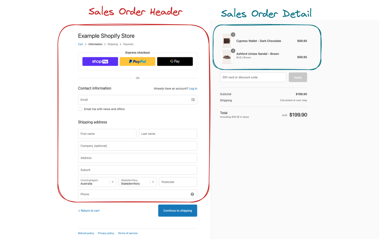
There are two tables in the sales schema that catch our attention. These two tables can be used to create the fact table for the sales process:
- The
sales.salesorderheadertable contains information about the credit card used in the order, the shipping address, and the customer. Each record in this table represents an order header that contains one or more order details. - The
sales.salesorderdetailtable contains information about the product that was ordered, and the order quantity and unit price, which we can use to calculate the revenue. Each record in this table represents a single order detail.
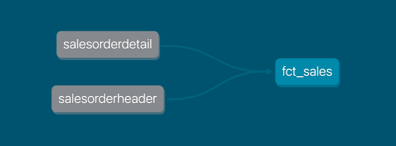
Let’s define a fact table called fct_sales which joins sales.salesorderheader and sales.salesorderdetail together. Each record in the fact table (also known as the grain) is an order detail.
Dimension tables
Dimension tables are used to represent contextual or descriptive information for a business process event. Examples of dimensions include:
- Customer details: Who is the customer for a particular order number?
- Website click location details: Which button is the user clicking on?
- Product details: What are the details of the product that was added to the cart?
Based on the business questions that our business user would like answered, we can identify several tables that would contain useful contextual information for our business process:
person.addressperson.countryregionproduction.productproduction.productcategorysales.customersales.store- And many more …
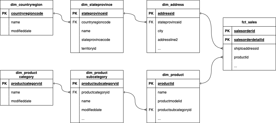
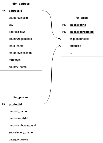
There are different ways we could create the dimension tables. We could use the existing relationships between the tables as depicted in the diagram below.
This is known as a snowflake schema design, where the fact table is the centre of the snowflake, and there are many fractals branching off the centre of the snowflake. However, this results in many joins that need to be performed by the consumer of the dimensional model.
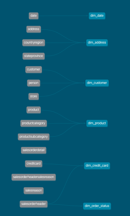
Instead, we can denormalize the dimension tables by performing joins.
This is known as a star schema and this approach reduces the amount of joins that need to be performed by the consumer of the dimensional model.
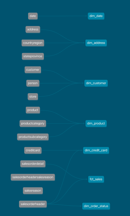
Using the star schema approach, we can identify 6 dimensions as shown below that will help us answer the business questions:
dim_product: a dimension table that joinsproduct,productsubcategory,productcategorydim_address: a dimension table that joinsaddress,stateprovince,countryregiondim_customer: a dimension table that joinscustomer,person,storedim_credit_card: a dimension table created fromcreditcarddim_order_status: a dimension table created by taking distinct statuses fromsalesorderheaderdim_date: a specially generated dimension table containing date attributes using the dbt_date package.
We have manually seeded the dim_date table since DuckDB is not supported by the dbt_date package.
In the next part, we use dbt to create the fact and dimension tables we have identified.
Part 4: Create the dimension tables
Let's first create dim_product . The other dimension tables will use the same steps that we’re about to go through.
Step 1: Create model files
Let’s create the new dbt model files that will contain our transformation code. Under adventureworks/models/marts/ , create two files:
dim_product.sql: This file will contain our SQL transformation code.dim_product.yml: This file will contain our documentation and tests fordim_product.
adventureworks/models/
└── marts
    ├── dim_product.sql
    ├── dim_product.yml
Step 2: Fetch data from the upstream tables
In dim_product.sql, you can select data from the upstream tables using Common Table Expressions (CTEs).
with stg_product as (
    select *
    from {{ ref('product') }}
),

stg_product_subcategory as (
    select *
    from {{ ref('productsubcategory') }}
),

stg_product_category as (
    select *
    from {{ ref('productcategory') }}
)

...
We use the ref function to reference the upstream tables and create a Directed Acyclic Graph (DAG) of the dependencies.
Step 3: Perform the joins
Next, perform the joins between the CTE tables using the appropriate join keys.
...

select
    ...
from stg_product
left join stg_product_subcategory on stg_product.productsubcategoryid = stg_product_subcategory.productsubcategoryid
left join stg_product_category on stg_product_subcategory.productcategoryid = stg_product_category.productcategoryid
Step 4: Create the surrogate key
Surrogate keys provide consumers of the dimensional model with an easy-to-use key to join the fact and dimension tables together, without needing to understand the underlying business context.
There are several approaches to creating a surrogate key:
- Hashing surrogate key: a surrogate key that is constructed by hashing the unique keys of a table (e.g.
md5(key_1, key_2, key_3)). - Incrementing surrogate key: a surrogate key that is constructed by using a number that is always incrementing (e.g.
row_number()). - Concatenating surrogate key: a surrogate key that is constructed by concatenating the unique key columns (e.g.
concat(key_1, key_2, key_3)).
We are using arguably the easiest approach which is to perform a hash on the unique key columns of the dimension table. This approach removes the hassle of performing a join with dimension tables when generating the surrogate key for the fact tables later.
To generate the surrogate key, we use a dbt macro that is provided by the dbt_utils package called generate_surrogate_key() . The generate surrogate key macro uses the appropriate hashing function from your database to generate a surrogate key from a list of key columns (e.g. md5(), hash()). Read more about the generate_surrogate_key macro.
...

select
    {{ dbt_utils.generate_surrogate_key(['stg_product.productid']) }} as product_key,
    ...
from stg_product
left join stg_product_subcategory on stg_product.productsubcategoryid = stg_product_subcategory.productsubcategoryid
left join stg_product_category on stg_product_subcategory.productcategoryid = stg_product_category.productcategoryid
Step 5: Select dimension table columns
You can now select the dimension table columns so that they can be used in conjunction with the fact table later. We select columns that will help us answer the business questions identified earlier.
...

select
    {{ dbt_utils.generate_surrogate_key(['stg_product.productid']) }} as product_key,
    stg_product.productid,
    stg_product.name as product_name,
    stg_product.productnumber,
    stg_product.color,
    stg_product.class,
    stg_product_subcategory.name as product_subcategory_name,
    stg_product_category.name as product_category_name
from stg_product
left join stg_product_subcategory on stg_product.productsubcategoryid = stg_product_subcategory.productsubcategoryid
left join stg_product_category on stg_product_subcategory.productcategoryid = stg_product_category.productcategoryid
Step 6: Choose a materialization type
You may choose from one of the following materialization types supported by dbt:
- View
- Table
- Incremental
It is common for dimension tables to be materialized as table or view since the data volumes in dimension tables are generally not very large. In this example, we have chosen to go with table, and have set the materialization type for all dimensional models in the marts schema to table in dbt_project.yml
models:
  adventureworks:
    marts:
      +materialized: table
      +schema: marts
Step 7: Create model documentation and tests
Alongside our dim_product.sql model, we can populate the corresponding dim_product.yml file to document and test our model.
version: 2

models:
  - name: dim_product
    columns:
      - name: product_key
        description: The surrogate key of the product
        tests:
          - not_null
          - unique
      - name: productid
        description: The natural key of the product
        tests:
          - not_null
          - unique
      - name: product_name
        description: The product name
        tests:
          - not_null
Step 8: Build dbt models
Execute the dbt run and dbt test commands to run and test your dbt models:
dbt run && dbt test
We have now completed all the steps to create a dimension table. We can now repeat the same steps to all dimension tables that we have identified earlier. Make sure to create all dimension tables before moving on to the next part.
Part 5: Create the fact table
After we have created all required dimension tables, we can now create the fact table for fct_sales.
Step 1: Create model files
Let’s create the new dbt model files that will contain our transformation code. Under adventureworks/models/marts/ , create two files:
fct_sales.sql: This file will contain our SQL transformation code.fct_sales.yml: This file will contain our documentation and tests forfct_sales.
adventureworks/models/
└── marts
    ├── fct_sales.sql
    ├── fct_sales.yml
Step 2: Fetch data from the upstream tables
To answer the business questions, we need columns from both salesorderheader and salesorderdetail. Let’s reflect that in fct_sales.sql :
with stg_salesorderheader as (
    select
        salesorderid,
        customerid,
        creditcardid,
        shiptoaddressid,
        status as order_status,
        cast(orderdate as date) as orderdate
    from {{ ref('salesorderheader') }}
),

stg_salesorderdetail as (
    select
        salesorderid,
        salesorderdetailid,
        productid,
        orderqty,
        unitprice,
        unitprice * orderqty as revenue
    from {{ ref('salesorderdetail') }}
)

...
Step 3: Perform joins
The grain of the fct_sales table is one record in the SalesOrderDetail table, which describes the quantity of a product within a SalesOrderHeader. So we perform a join between salesorderheader and salesorderdetail to achieve that grain.
...

select
    ...
from stg_salesorderdetail
inner join stg_salesorderheader on stg_salesorderdetail.salesorderid = stg_salesorderheader.salesorderid
Step 4: Create the surrogate key
Next, we create the surrogate key to uniquely identify each row in the fact table. Each row in the fct_sales table can be uniquely identified by the salesorderid and the salesorderdetailid which is why we use both columns in the generate_surrogate_key() macro.
...

select
    {{ dbt_utils.generate_surrogate_key(['stg_salesorderdetail.salesorderid', 'salesorderdetailid']) }} as sales_key,
		...
from stg_salesorderdetail
inner join stg_salesorderheader on stg_salesorderdetail.salesorderid = stg_salesorderheader.salesorderid
Step 5: Select fact table columns
You can now select the fact table columns that will help us answer the business questions identified earlier. We want to be able to calculate the amount of revenue, and therefore we include a column revenue per sales order detail which was calculated above by unitprice * orderqty as revenue .
...

select
    {{ dbt_utils.generate_surrogate_key(['stg_salesorderdetail.salesorderid', 'salesorderdetailid']) }} as sales_key,
    stg_salesorderdetail.salesorderid,
    stg_salesorderdetail.salesorderdetailid,
    stg_salesorderdetail.unitprice,
    stg_salesorderdetail.orderqty,
    stg_salesorderdetail.revenue
from stg_salesorderdetail
inner join stg_salesorderheader on stg_salesorderdetail.salesorderid = stg_salesorderheader.salesorderid
Step 6: Create foreign surrogate keys
We want to be able to slice and dice our fact table against the dimension tables we have created in the earlier step. So we need to create the foreign surrogate keys that will be used to join the fact table back to the dimension tables.
We achieve this by applying the generate_surrogate_key() macro to the same unique id columns that we had previously used when generating the surrogate keys in the dimension tables.
...

select
    {{ dbt_utils.generate_surrogate_key(['stg_salesorderdetail.salesorderid', 'salesorderdetailid']) }} as sales_key,
    {{ dbt_utils.generate_surrogate_key(['productid']) }} as product_key,
    {{ dbt_utils.generate_surrogate_key(['customerid']) }} as customer_key,
    {{ dbt_utils.generate_surrogate_key(['creditcardid']) }} as creditcard_key,
    {{ dbt_utils.generate_surrogate_key(['shiptoaddressid']) }} as ship_address_key,
    {{ dbt_utils.generate_surrogate_key(['order_status']) }} as order_status_key,
    {{ dbt_utils.generate_surrogate_key(['orderdate']) }} as order_date_key,
    stg_salesorderdetail.salesorderid,
    stg_salesorderdetail.salesorderdetailid,
    stg_salesorderdetail.unitprice,
    stg_salesorderdetail.orderqty,
    stg_salesorderdetail.revenue
from stg_salesorderdetail
inner join stg_salesorderheader on stg_salesorderdetail.salesorderid = stg_salesorderheader.salesorderid
Step 7: Choose a materialization type
You may choose from one of the following materialization types supported by dbt:
- View
- Table
- Incremental
It is common for fact tables to be materialized as incremental or table depending on the data volume size. As a rule of thumb, if you are transforming millions or billions of rows, then you should start using the incremental materialization. In this example, we have chosen to go with table for simplicity.
Step 8: Create model documentation and tests
Alongside our fct_sales.sql model, we can populate the corresponding fct_sales.yml file to document and test our model.
version: 2

models:
  - name: fct_sales
    columns:

      - name: sales_key
        description: The surrogate key of the fct sales
        tests:
          - not_null
          - unique

      - name: product_key
        description: The foreign key of the product
        tests:
          - not_null

      - name: customer_key
        description: The foreign key of the customer
        tests:
          - not_null

      ...

      - name: orderqty
        description: The quantity of the product
        tests:
          - not_null

      - name: revenue
        description: The revenue obtained by multiplying unitprice and orderqty
Step 9: Build dbt models
Execute the dbt run and dbt test commands to run and test your dbt models:
dbt run && dbt test
Great work, you have successfully created your very first fact and dimension tables! Our dimensional model is now complete!! 🎉
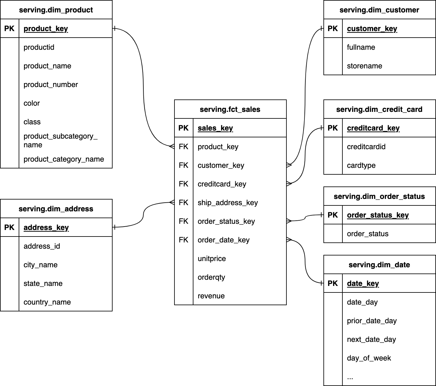
Part 6: Document the dimensional model relationships
Let’s make it easier for consumers of our dimensional model to understand the relationships between tables by creating an Entity Relationship Diagram (ERD).
The ERD will enable consumers of our dimensional model to quickly identify the keys and relationship type (one-to-one, one-to-many) that need to be used to join tables.
Part 7: Consume dimensional model
Finally, we can consume our dimensional model by connecting our data warehouse to our Business Intelligence (BI) tools such as Tableau, Power BI, and Looker.
Most modern BI tools have a built-in semantic layer that supports relationships between tables, which is required if we want to consume the dimensional models directly without any additional data transformation.
In Looker for example, we can define relationships using LookML:
explore: fct_order {
  join: dim_user {
    sql_on: ${fct_order.user_key} = ${dim_user.user_key} ;;
    relationship: many_to_one
  }
}
If your BI tool doesn’t have a semantic layer that supports relationships, then you will have to reflect that relationship by creating a One Big Table (OBT) that joins the fact table against all of its dimension tables.
with f_sales as (
    select * from {{ ref('fct_sales') }}
),

d_customer as (
    select * from {{ ref('dim_customer') }}
),

d_credit_card as (
    select * from {{ ref('dim_credit_card') }}
),

d_address as (
    select * from {{ ref('dim_address') }}
),

d_order_status as (
    select * from {{ ref('dim_order_status') }}
),

d_product as (
    select * from {{ ref('dim_product') }}
),

d_date as (
    select * from {{ ref('dim_date') }}
)

select
    {{ dbt_utils.star(from=ref('fct_sales'), relation_alias='f_sales', except=[
        "product_key", "customer_key", "creditcard_key", "ship_address_key", "order_status_key", "order_date_key"
    ]) }},
    {{ dbt_utils.star(from=ref('dim_product'), relation_alias='d_product', except=["product_key"]) }},
    {{ dbt_utils.star(from=ref('dim_customer'), relation_alias='d_customer', except=["customer_key"]) }},
    {{ dbt_utils.star(from=ref('dim_credit_card'), relation_alias='d_credit_card', except=["creditcard_key"]) }},
    {{ dbt_utils.star(from=ref('dim_address'), relation_alias='d_address', except=["address_key"]) }},
    {{ dbt_utils.star(from=ref('dim_order_status'), relation_alias='d_order_status', except=["order_status_key"]) }},
    {{ dbt_utils.star(from=ref('dim_date'), relation_alias='d_date', except=["date_key"]) }}
from f_sales
left join d_product on f_sales.product_key = d_product.product_key
left join d_customer on f_sales.customer_key = d_customer.customer_key
left join d_credit_card on f_sales.creditcard_key = d_credit_card.creditcard_key
left join d_address on f_sales.ship_address_key = d_address.address_key
left join d_order_status on f_sales.order_status_key = d_order_status.order_status_key
left join d_date on f_sales.order_date_key = d_date.date_key
In the OBT above, we perform joins between the fact and dimension tables using the surrogate keys.
Using dbt_utils.star(), we select all columns except the surrogate key columns since the surrogate keys don't hold any meaning besides being useful for the joins.
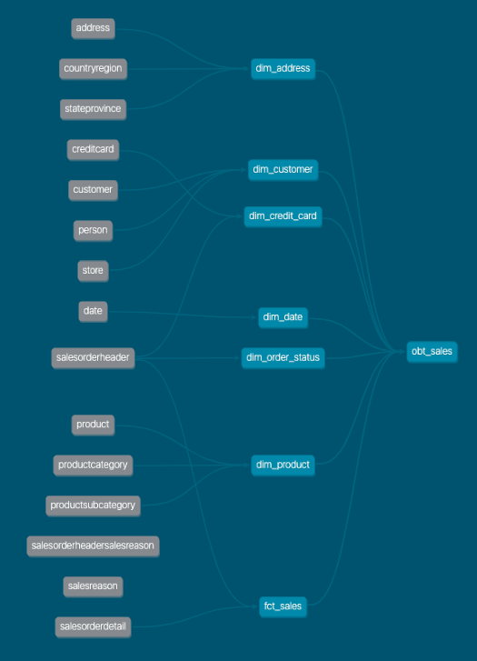
We can then build the OBT by running dbt run. Your dbt DAG should now look like this:
Congratulations, you have reached the end of this tutorial. If you want to learn more, please see the learning resources below on dimensional modeling.
Learning resources
- Kimball group learning resources
- The Data Warehouse toolkit book
- dbt discourse on whether dimensional modeling is still relevant
- dbt glossary on dimensional modeling
If you have any questions about the material, please reach out to me on the dbt Community Slack (@Jonathan Neo), or on LinkedIn.
Author's note: The materials in this article were created by Data Engineer Camp, a 16-week data engineering bootcamp for professionals looking to transition to data engineering and analytics engineering. The article was written by Jonathan Neo, with editorial and technical guidance from Kenny Ning and editorial review from Paul Hallaste and Josh Devlin.




Comments